Definition: Model Bias & Model Variance

Bias	Variance
Assumptions that we make on ‘Data’ Boosting Method to Minimize	Variance in Data Set Bagging Method to Minimize sensitivity of data

* The Error we get during the training phase is called BIAS

(3 Eg: Bias for 11th Degree Polynomial is 0, Bias for Plane(linear Model) is High)

• We want a Model with Low Variance and Low Bias
• We want to choose model which has less SENSITIVITY to the Variance data
• Objective of Ensembles: To Minimize Bias & Variance

Supervised Learning:

f(x) –> y

f: Function x:input variable –>: Maps y: output label

Supervised Machine Learning is all about ‘Learning a Function’, that maps input(x) to output(y)

This Function could be Regression or Discriminant(Classification)

In supervised learning, we do ‘inductive learning’.

But, Incase of Unsupervised learning, we only have input(x).

Predominant Task under Unsupervised Learning is CLUSTERING.

(Others are ‘Association Mining’, ‘Representation Learning’, ‘Distribution Learning’

Type of Data

• Names of people: String
• Classroom test marks: Matrix (Eg: 50 Students, 6 Subjects, 50*6 Matrix)
• Census Data: Table Data
• ECG: Need to transform data, to wave form, 1D Time Series Data
• Video: Time Series with Matrix
• Song: Time Series with (Sterio: 2 Channel, DolbyAtmos:9 Channel)

—

3 Sample Temperature Data: (9AM, 27* C), (11AM, 32*C), (12PM, 23*C) – Which Dimension is this Data?

• In this there is a Time Feature and Temperature Feature , so Dimensionality is = No. of Features (No of Columns)
• The Data Set is arranged as a Matrix, “ ROWS=Samples, Columns are Features”,
• Every Column is Feature Column , Every Row is ‘ DATA INSTANCE’
• ‘n’ rows and ‘p’ columns :- defined in most books, so this matrix is n*p
• d1: { 9 | 27 } , 1D Vector of Size 2
• d2: { 11 | 32 } ;;; d3{ 12, 32 } , Although it appears 2 column, its actually 3 Column, for AM|PM (Meridian)
• Or the other way is to transform ‘AM|PM’ 12Hrs Format data to ‘24Hrs’ Format data to remove ambiguity still with 2 Columns
• While Transforming Data, think intelligently representing ‘Numeric’ to perform arithmetic operations or identify ‘Best Representation’ to make our life simpler..!
• For AM|PM/ Categorical data, do ‘ONE HOT ENCODING’

	a	p
a	1	0
p	0	1

• Above is for 2, for many columns, this matrix would be wider,
• With One Hot Encoding, the same temperature data set would become 4 Columns,
• ‘One Hot Encoding’ is one style, another one is Encoded 1, Eg: Monday:000, Tue:001, Wed:010…

First Stage of Data Preparation:

1. First Stage: Preprocessing
2. Second Stage: Normalization

In order to not get affected Euclidean Distance, make Scale Factor of every dimension to be uniform

Curse of Dimensionality: When we have more dimensions (10, 10^2, 10^3..)

Interpretability of the Euclidean Distance measure itself has gone

Vector Addition: Just by Extending , Vector Subtraction: Create a mirror and add.

For (data) ‘Similarity’, Angle is what we need to pay attention to..!

2 Data Points : Cos0: 1 => Closer, Cos90:0 => Dissimilar

This is called COSINE SIMILARITY

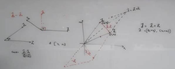
But still interpretation of Vector Addition is Subject to Domain!

KNN

Analogy: Like person sitting in the classroom, next to each other – by choosing to sit in the next class.

To Choose Neighborhood: Eg: Age, Gender, Language, Field of Work, Proximity to AC Cooling, Average InTime,

Cluster:

Attribute Data, Relational Data, Networked(both) Data

Def: Vantage Point: Is a point of view from where we see: is very important

Sensitivity/Resolution of (Euclidean) measure is controlled by Threshold that we set.

We can figure out the ‘Threshold’ value by Cross Validation

K-Means Cluster

(is motivated by KNN, same idea)

Discover cluster based on the No. given

• Eg: Start with 3 starting points(membership), called “Centroids”
• Centroid:= Average of Data Points (in the cluster)
• It aims to find ‘K’ Centroids by estimating ‘Potential Clusters’
• Recompute the Centroid, for the new cluster that is formed and repeat.
• We stop repeating the algorithm, when centroids stop moving
• Big Disadvantage: K-Means is too sensitive to outliers (Solution: K-Medoids)
• 2nd Disadvantage of K-Means, we don’t know ‘K’, we need to do educated guess
• 3rd Disadvantage: If more overlapping data points, repeatability of cluster is not possible, due to initial random centroid selection
• “Intra-Cluster Average Distance” should be minimum – called INERTIA
• “Inter-Cluster Average Distance” should be Maximum
• Linear Search: The parameter we’re passing the value in Python: cluster_range = range( 1, 15 )
• If Data(D) is large, draw sample data(D’) & find K-Centroid – For Very Large Data Sets.
• K-Means only works for ‘CONVEX Clusters’. – Another Limitation (Convex: Like potato)

When to Choose, Convex/Non-Convex: By Data-Characterization, ie studying various aspects of data.

Weakness of k-means:

The k-means algorithm is not suitable for discovering clusters that are not hyper-ellipsoids (or hyper-spheres)

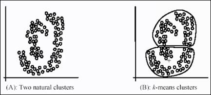
The premise of K-means is to create convex clusters – which does not make sense for above.

So we should have another technique – aiming at DENSE REGIONS.

& that technique is called DBScan

DBScan is a greedy algorithm – it will try to find continuous dense regions.

• Define a quantity called ‘E’ Epsilon , using this quantity define a circle

Epsilon Boundary:

How best to find epsilon boundary? We’ve to repeat the experiment

Border Points: & Min.Points

• DB Scan assumes uniform density across data points
• Data points like this is challenging/setback for DBScan:

Kmeans ++ -> To identify the best k (with ‘k=auto’ in python )

In UnSupervised learning, we have to be very CREATIVE…!

SoftClustering methods: Fuzzy C-Means which allows overlapping of data points across clusters

• K-Means algorithm is under “Partitioning Methods” (Divide data)
• “Density Methods” : DBScan
• “Hierarchical Methods” – drilling down,2 way: 1. Divisive, 2. Agglomerative Style (Popular method)

Agglomerative Style: Start with every data point as cluster , then objective is to merge clusters which are closer to each other

With “Single(Chain) / Complete(Convex) / Average” Linkage

Dendrogram: Tree Like diagram for Hierarchical – Agglomerative Style

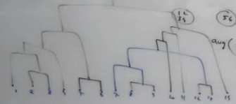
We Can cut and choose what granularity level of cluster we want – Advantage of Hierarchical Cluster.

The model is not dependent on the parameter.

We can spawn Python THREAD, to have parallel operation for Agglomerative Clustering

Support Vector Machines

Find Optimal Hyperplane , with slab of width m.

1. Objective of SVM is to identify Single Unique Decision Boundary
2. Identify a Slab instead of Decision Margin
3. The Slack ‘C’: Allow some points to move across the decision surface
4. The model is only dependent on the support point